Camera Matching

Camera matching is the technique that allows to compute the position, rotation and focal length of the camera that shot a given photo. This process has some useful usecases:

Recreating a 3D scene starting from a 2D image. When creating 3D assets of organic objects, the artist uses reference photos to guide his creative process, but this works up to a certain point. Instead, when the meshes are mainly geometric (like most of the buildings), the photo can be superimposed to the scene being created so that the $x$, $y$ and $z$ axes match those of the image, greatly simplifying the process.
Measure relative objects sizes. This helps for example if we would like to know the dimensions of object that are visible but difficult to reach. Another field of application is the forensic image analysis of photographic evidences.
Create the illusion of a 3D set from a flat landscape. Instead of creating a complex scene background using a 3D modeling tool, we can obtain a more realistic result using a photo. To avoid making the landscape look flat, we can project it on a simple geometry that roughly reproduces the changing depth of the different picture regions. This technique helps speed up the process of collimating the panorama with the underlying geometry.

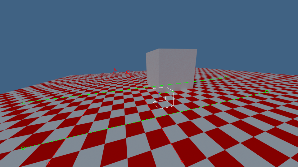
To see how this is possible, we have to understand some simple concepts. As reference we will use the following image: The reference images we will use throughout the exercise. It consists of:

A $x$-$y$ plane with a checkerboard pattern oriented following the $x$ and $y$ direction
Two red segments that in the scene are parallel to the $x$ axis.
The green strokes that extend in the $y$ direction
A blue circle at the cube corner. It corresponds to the position of the axes origin the scene

A fundamental property of perspective is what is called the “vanishing point”: all the lines that in the 3D scene are parallel to each other, in the photo converge in the same point. Looking at the reference image it’s evident that the two red lines that follow the edges of the checkerboard pattern converge at a (vanishing) point about in the middle of the picture. It’s easy to prove that using linear algebra. Let’s consider all the lines with direction $\vec{d}$:

$\vec{x}=\vec{x}_0 + \lambda \vec{d}$

and a generic projection matrix $C$. If we follow this line ad infinitum, the projection of our position will converge to the point:

$\begin{align*} \vec{y} &= \lim_{\lambda \to \infty} C \vec{x} \\ \vec{y} &= \lim_{\lambda \to \infty} C \left( \vec{x}_0 + \lambda \vec{d} \right) \end{align*}$

Thanks to the fact that we are using homogeneous coordinates, we can scale the vector using any non-zero coefficient (in our case $\frac{1}{\lambda}$) without influencing the result:

$\begin{align*} \vec{y}_s &= \lim_{\lambda \to \infty} \frac{1}{\lambda} C \left( \vec{x}_0 + \lambda \vec{d} \right) \\ \vec{y}_s &= \lim_{\lambda \to \infty} C \left( \frac{1}{\lambda}\vec{x}_0 + \vec{d} \right) \\ \vec{y}_s &= C \vec{d} \end{align*}$

This shows that the point projection converges to a coordinate that depends only from the movement direction. In the above picture we can arbitrarily choose that the red segments are going in the $x$ direction and we can measure that the coordinates (taken from the optical center, i.e. the middle of the image) at which they converge are $\left( -89, 71 \right)$, so it holds that:

$C \begin{bmatrix} 1 \\ 0 \\ 0 \\ 0 \end{bmatrix} = \alpha_1 \begin{bmatrix} -89 \\ 71 \\ 1 \end{bmatrix}$

Once again, the $\alpha_1$ term is necessary because we are working with homogeneous coordinates. From basic linear algebra we already know that this means that the first column of the projection matrix must be parallel to $\left[ -89, 71, 1 \right]^T$. We repeat the same procedure for the $y$ axis, that we choose to be parallel to the green segments. We see that prolonging those edges we reach the point $\left( 947, 104 \right)$, so:

$C \begin{bmatrix} 0 \\ 1 \\ 0 \\ 0 \end{bmatrix} = \alpha_2 \begin{bmatrix} 947 \\ 104 \\ 1 \end{bmatrix}$

At this point we have enough data to compute the focal length of the camera. To do that, we have to decompose the projection matrix in a sequence of a translation, a rotation and a projection normal to the $x$-$y$ plane:

$\begin{align*} C &= \begin{bmatrix} 1 & 0 & 0 & 0 \\ 0 & 1 & 0 & 0 \\ 0 & 0 & -1/f & 0 \\ \end{bmatrix} \begin{bmatrix} R & 0 \\ 0 & 1 \\ \end{bmatrix} \begin{bmatrix} I & -t \\ 0 & 1 \\ \end{bmatrix} \\ C &= \begin{bmatrix} 1 & 0 & 0 & 0 \\ 0 & 1 & 0 & 0 \\ 0 & 0 & -1/f & 0 \\ \end{bmatrix} \begin{bmatrix} R & -Rt \\ 0 & 1 \\ \end{bmatrix} \\ C &= \begin{bmatrix} 1 & 0 & 0 \\ 0 & 1 & 0 \\ 0 & 0 & -1/f \\ \end{bmatrix} \begin{bmatrix} R & -Rt \\ \end{bmatrix} \end{align*}$

Substituting $C$ with the values we found leveraging the vanishing points, we come to the following equation:

$\begin{align*} \begin{bmatrix} -89 \alpha_1 & 947 \alpha_2 & \square & \square \\ 71 \alpha_1 & 104 \alpha_2 & \square & \square \\ \alpha_1 & \alpha_2 & \square & \square \end{bmatrix} &= \begin{bmatrix} 1 & 0 & 0 \\ 0 & 1 & 0 \\ 0 & 0 & -1/f \\ \end{bmatrix} \begin{bmatrix} R & -Rt \\ \end{bmatrix} \\ \begin{bmatrix} -89 \alpha_1 & 947 \alpha_2 & \square & \square \\ 71 \alpha_1 & 104 \alpha_2 & \square & \square \\ -f \alpha_1 & -f \alpha_2 & \square & \square \end{bmatrix} &= \begin{bmatrix} R & -Rt \\ \end{bmatrix} \end{align*}$

As all the rotation matrices, $R$ is orthonormal, so the first two columns of the matrix on the left side must be orthogonal, i.e.:

$\begin{align*} \alpha_1 \begin{bmatrix} -89 \\ 71 \\ -f \end{bmatrix} \alpha_2 \begin{bmatrix} 947 \\ 104 \\ -f \end{bmatrix} &= 0 \\ \begin{bmatrix} -89 \\ 71 \\ -f \end{bmatrix} \begin{bmatrix} 947 \\ 104 \\ -f \end{bmatrix} &= 0 \\ f^2 &= - \begin{bmatrix} -89 \\ 71 \end{bmatrix} \begin{bmatrix} 947 \\ 104 \end{bmatrix} \\ f &= 227 \end{align*}$

That is equivalent to a horizontal aperture angle of:

$\beta = 2 \arctan \left( \frac{w}{2f} \right) = 120^\circ$

Where $w$ is the image width, in pixel (if we are interested in the vertical field of view, use the image height instead). Now that we know $f$, we can choose $\alpha_1$ and $\alpha_2$ so that the two columns have unitary norm:

$\begin{bmatrix} -0.297 & 0.954 & \square & \square \\ 0.237 & 0.105 & \square & \square \\ -0.925 & -0.279 & \square & \square \end{bmatrix} = \begin{bmatrix} R & -Rt \\ \end{bmatrix}$

$R$, like any other orthogonal matrix, the third column must be the cross product of the first two:

$\begin{bmatrix} -0.297 & 0.954 & 0.031 & \square \\ 0.237 & 0.105 & -0.965 & \square \\ -0.925 & -0.279 & 0.257 & \square \end{bmatrix} = \begin{bmatrix} R & -Rt \\ \end{bmatrix}$

We can multiply again both sides by the $x$-$y$ projection matrix:

$\begin{bmatrix} -0.297 & 0.954 & 0.031 & \square \\ 0.237 & 0.105 & -0.966 & \square \\ 0.003 & 0.001 & 0.001 & \square \end{bmatrix} = \begin{bmatrix} 1 & 0 & 0 \\ 0 & 1 & 0 \\ 0 & 0 & -1/f \\ \end{bmatrix} \begin{bmatrix} R & -Rt \\ \end{bmatrix}$

To find the correct values for the fourth column, we can ask the user to tell us where the origin of the axes must be projected. For our reference image we could choose the corner of the grey cube that is highlighted by a small blue circle, that is at $\left( 31, -33 \right)$. We can thus remove 2 additional unknowns from the matrix $C$ because:

$C \begin{bmatrix} 0 \\ 0 \\ 0 \\ 1 \end{bmatrix} = \alpha_3 \begin{bmatrix} 31 \\ -33 \\ 1 \\ \end{bmatrix}$

The value of $\alpha_3$ can be set to any value, if we have no data about the size of the elements on the scene. If instead we know for example that the side corner of the cube is 1 meter high and on the image it is 146 pixel long, we can add:

$C \begin{bmatrix} 0 \\ 0 \\ 1 \\ 1 \end{bmatrix} = \begin{bmatrix} 0.031 \\ -0.966 \\ 0.001 \\ \end{bmatrix} + \alpha_3 \begin{bmatrix} 31 \\ -33 \\ 1 \\ \end{bmatrix}$

And impose:

$\left( 31 - \frac{0.031 + 31 \alpha_3}{0.001 + \alpha_3} \right)^2 + \left( -33 - \frac{-0.966 - 33 \alpha_3}{0.001 + \alpha_3} \right)^2 = 146^2$

The solution $\alpha_3 = 0.005$ let us complete the projection matrix as follows:

$C = \begin{bmatrix} -0.297 & 0.954 & 0.031 & 0.170 \\ 0.237 & 0.105 & -0.966 & -0.181 \\ 0.003 & 0.001 & 0.001 & 0.005 \end{bmatrix}$

Having the $C$ matrix completely defined allow us to extract all the other useful parameters like the camera position $\left( -1.312,-0.568, -0.571 \right)$ and rotation angles $\left( -104.910^\circ, -1.763^\circ, 107.280^\circ \right)$. This entire algorithm can be executed using this Octave script that I have developed to compute the above values. You can now extend, customize and start using it together with your favorite 3D modeling software. Enjoy!